System Design Phase 1 — Part 8: Back-of-the-Envelope Estimation
📚 Table of Contents
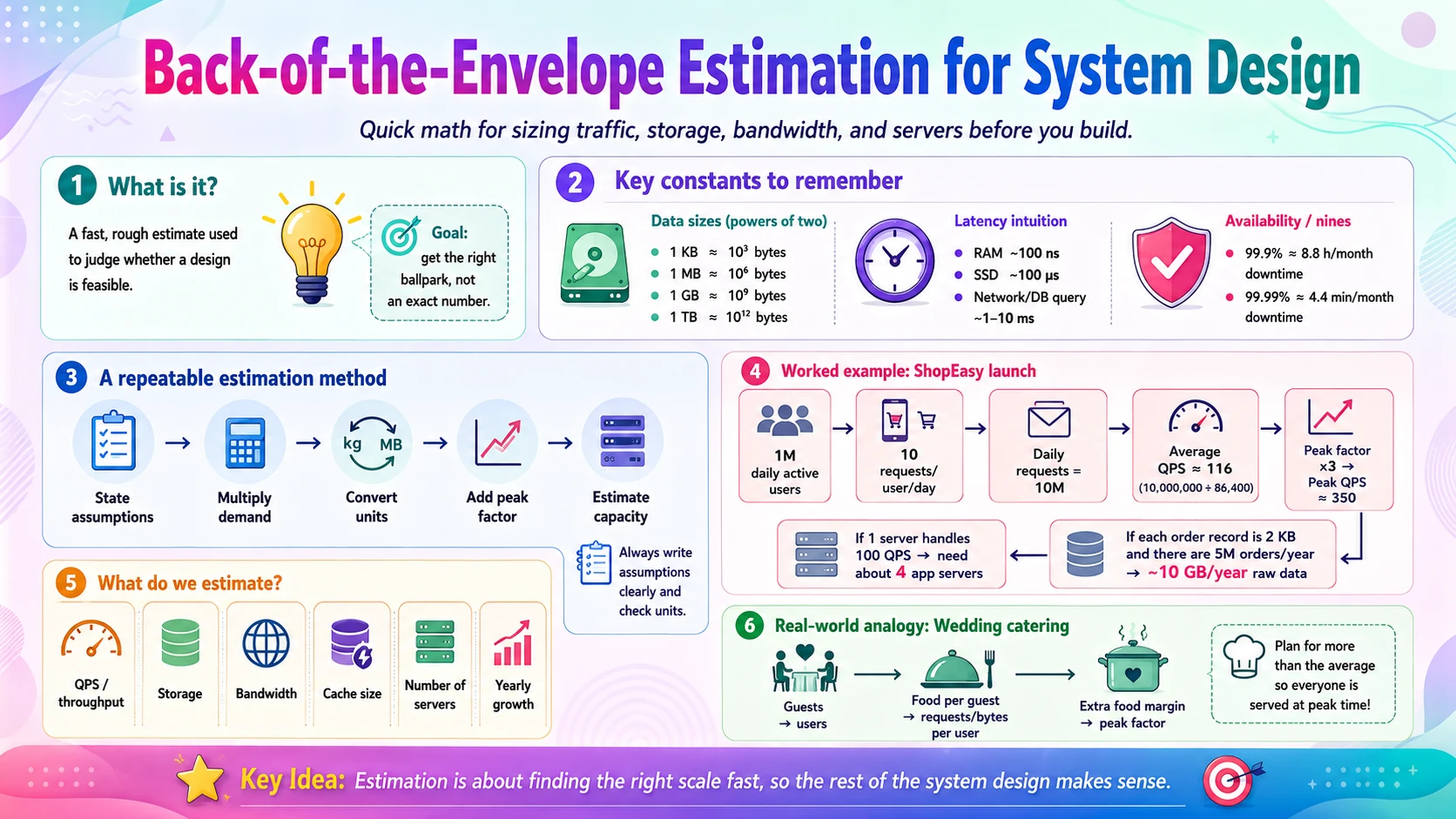
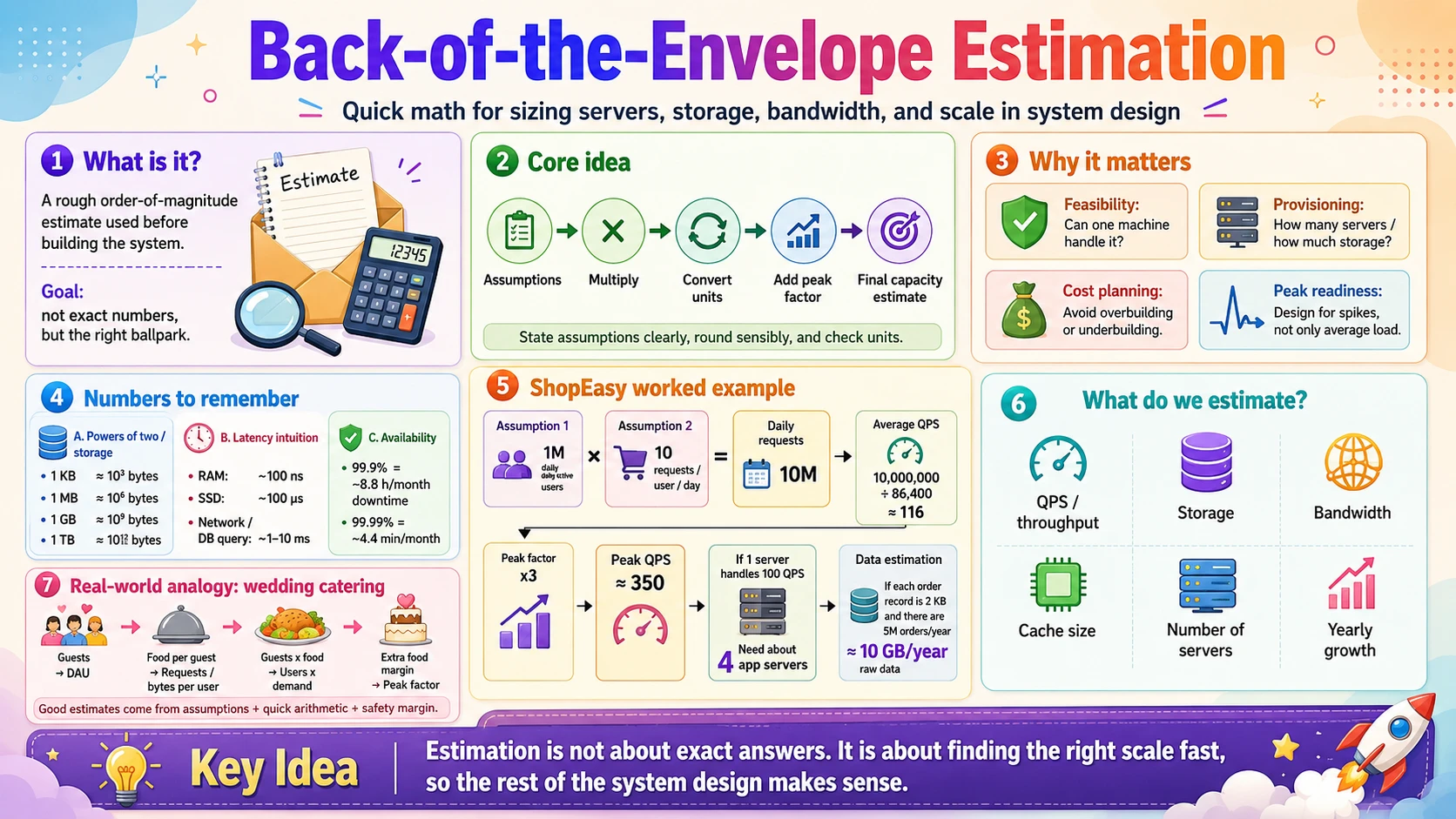
Before you commit to an architecture, you need a rough sense of the numbers it must handle: how many requests per second, how much storage per year, how much bandwidth, how many servers. Back-of-the-envelope estimation is the skill of producing those numbers quickly with simple math and a few memorised constants — no spreadsheets, no benchmarks, just enough accuracy to tell whether a design is sensible. This post is a single, flowing walkthrough of the whole skill. You will learn the powers of two that define data units, the latency numbers every programmer should know, how availability is measured in "nines" and tied to SLAs, and a repeatable method for estimating daily active users, QPS, peak traffic, storage, and bandwidth — finishing with a complete worked example. Everything is explained with real-world analogies, a diagram, and step-by-step math, starting from zero.
🧮 1. Back-of-the-Envelope Estimation
This is the one Phase 1 topic that is a single flowing subject rather than a set of separate sub-topics. It builds in order: first the raw ingredients every estimate relies on — powers of two, latency numbers, and availability numbers — then the step-by-step method for turning a few assumptions into capacity numbers, and finally a full worked example estimating QPS and storage.
1.1 🎯 Introduction
Imagine you're planning the infrastructure for our online store ShopEasy before a big launch. Someone asks: "How many servers do we need? How much database storage for a year? Will one cache fit in memory?" You don't have real traffic yet, and you can't run a benchmark on a system that doesn't exist. What you can do is reason it out on the back of an envelope — a few assumptions, some simple multiplication, and a handful of numbers you've memorised — and arrive at an answer that's roughly right. That's back-of-the-envelope estimation.
As Google's Jeff Dean put it, back-of-the-envelope calculations are "estimates you create using a combination of thought experiments and common performance numbers to get a good feel for which designs will meet your requirements." The goal is never a precise figure — it's an order-of-magnitude answer: is this 10 servers or 10,000? 1 GB or 1 PB? That's usually enough to compare two designs and rule out the ones that can't possibly work.
To do this well, three things need to be second nature: the powers of two that define data sizes, the latency numbers that tell you how slow each operation is, and the availability numbers that translate a percentage like "99.99%" into real downtime. With those in hand, a simple method turns a few assumptions into a full capacity estimate. This post walks through all of it and ends with a complete worked example.
💡 Estimation is about the process, not the exact number. A good estimate shows clear assumptions, sensible rounding, and correct units. Two engineers estimating the same system should land in the same ballpark — that ballpark is what guides the design.
1.2 💡 Why It Matters
Estimation is what turns a vague idea into an engineering decision. Before writing a line of code, a rough calculation tells you whether the data fits on one machine or needs sharding, whether reads can be served from a cache, and how much the whole thing will cost to run. The numbers involved are huge and non-obvious: Twitter-scale services handle thousands of writes per second and tens of thousands at peak; five years of media can add up to tens of petabytes. Guessing wrong by an order of magnitude means either a system that falls over on day one or a cluster that costs 10× more than needed.
- Feasibility — a quick estimate reveals whether a design is even possible. If one machine can do 10,000 QPS and you need 700,000, you immediately know you need ~70 machines, not one.
- Provisioning — capacity numbers decide how many servers, how much storage, and how big a cache to allocate — and how much to budget.
- Comparing designs — estimates let you rule out approaches cheaply. A design that would need a petabyte of RAM is off the table before you build it.
- Planning for peaks — average load is not what breaks systems; the peak does. Estimation makes you size for the spike, not the average.
Why system design cares: almost every design starts by scoping the problem with numbers — DAU, QPS, storage, bandwidth. Those estimates drive every later choice: SQL vs NoSQL, single database vs sharded, cache or no cache, one region or many. Get the scale right and the rest of the design follows.
1.3 🏠 Real-world Analogy
Think about catering a wedding. You don't know exactly how many guests will show up or precisely how much each will eat — but you still have to order food and book a venue in advance. So you estimate: "About 200 guests. Say each eats roughly 0.5 kg of food — that's 100 kg. Drinks: 3 glasses each, 600 glasses. Round up for a safety margin." Nobody weighs every plate; a few reasonable assumptions and simple multiplication get you close enough to place the order confidently.
System estimation is exactly this. Guests become users, "how much each eats" becomes requests per user or bytes per item, and the safety margin becomes the peak factor you multiply by so you don't run out during the rush. You'd rather slightly over-cater than have guests go hungry — just as you'd rather provision for the traffic peak than crash during it.
| Wedding Catering | System Estimation | Meaning |
|---|---|---|
| 👰 Expected number of guests | 👥 Daily active users (DAU) | The size of the audience you serve |
| 🍽️ Food each guest eats | 📨 Requests / bytes per user | Per-unit demand you multiply out |
| 🧮 Guests × food per guest | ✖️ Users × requests per user | The core estimation multiplication |
| 🎉 Extra for the dinner rush | 📈 Peak factor (×2–×3) | Size for the spike, not the average |
| 📦 Total food to order & store | 💾 Storage & bandwidth to provision | What you must have ready in advance |
The caterer's skill isn't exact prediction — it's making sensible assumptions, doing quick arithmetic, and building in a margin. Every estimate in this post follows the same recipe: state assumptions, multiply, round, and pad for the peak.
1.4 📖 Key Terms
| Term | Simple Definition | Quick Example |
|---|---|---|
| MAU | Monthly Active Users — unique users in a month | 300 million |
| DAU | Daily Active Users — unique users in a day | 150 million |
| QPS | Queries (requests) Per Second the system handles | ~3,500 writes/sec |
| Peak QPS | QPS during the busiest period, not the average | 2 × average ≈ 7,000 |
| Throughput | Total work processed per unit time | Requests or MB per second |
| Storage | Total data kept on disk over time | ~55 PB over 5 years |
| Bandwidth | Data transferred per second (in or out) | ~347 MB/s of uploads |
| Read/Write ratio | How many reads occur per write | 100:1 (read-heavy) |
| Latency | Time for a single operation to complete | Disk seek ≈ 10 ms |
| Availability | % of time the system is operational | 99.99% ("four nines") |
| SLA | Service Level Agreement — promised uptime | Cloud providers ≥ 99.9% |
| Byte | 8 bits; one ASCII character = 1 byte | "A" = 1 byte |
1.5 🔢 How It Works
Estimation rests on three sets of numbers you should know cold — powers of two, latency numbers, and availability numbers — plus a repeatable method that turns assumptions into capacity. We'll cover each in turn.
A. Powers of Two & Data Units
Data volume is measured in bytes, and a byte is 8 bits (one ASCII character fits in a byte). Because computers are binary, storage units are powers of two, but for estimation you round them to the nearest power of ten — that's what makes the mental math easy. Memorise this table:
| Power of 2 | Approximate value | Full name | Short name |
|---|---|---|---|
| 210 | 1 Thousand | 1 Kilobyte | 1 KB |
| 220 | 1 Million | 1 Megabyte | 1 MB |
| 230 | 1 Billion | 1 Gigabyte | 1 GB |
| 240 | 1 Trillion | 1 Terabyte | 1 TB |
| 250 | 1 Quadrillion | 1 Petabyte | 1 PB |
So a thousand bytes ≈ 1 KB, a million ≈ 1 MB, a billion ≈ 1 GB, a trillion ≈ 1 TB, and a quadrillion ≈ 1 PB. Each step up is ×1,000. When an estimate produces "30 × 1012 bytes," you instantly read it as 30 TB.
B. Latency Numbers Every Programmer Should Know
These are the classic latency numbers published by Google's Dr. Jeff Dean. They let you reason about whether an operation is cheap (memory) or expensive (disk, cross-continent network) without measuring. The original 2010 numbers:
| Operation | Time |
|---|---|
| L1 cache reference | 0.5 ns |
| Branch mispredict | 5 ns |
| L2 cache reference | 7 ns |
| Mutex lock/unlock | 100 ns |
| Main memory reference | 100 ns |
| Compress 1 KB with Zippy | 10,000 ns = 10 µs |
| Send 2 KB over 1 Gbps network | 20,000 ns = 20 µs |
| Read 1 MB sequentially from memory | 250,000 ns = 250 µs |
| Round trip within the same datacenter | 500,000 ns = 500 µs |
| Disk seek | 10,000,000 ns = 10 ms |
| Read 1 MB sequentially from the network | 10,000,000 ns = 10 ms |
| Read 1 MB sequentially from disk | 30,000,000 ns = 30 ms |
| Send packet CA → Netherlands → CA | 150,000,000 ns = 150 ms |
📏 Units: ns = nanosecond, µs = microsecond, ms = millisecond. 1 ns = 10-9 s; 1 µs = 10-6 s = 1,000 ns; 1 ms = 10-3 s = 1,000 µs = 1,000,000 ns.
Hardware has improved since 2010. A 2020 visualisation of the same operations shows memory and SSD getting much faster, while the cross-continent network round trip barely changes (it's bounded by the speed of light):
| Operation (2020) | Time |
|---|---|
| L1 cache reference | 1 ns |
| Branch mispredict | 3 ns |
| L2 cache reference | 4 ns |
| Mutex lock/unlock | 17 ns |
| Send 2,000 bytes over commodity network | 44 ns |
| Main memory reference | 100 ns |
| Compress 1 KB with Zippy | 2,000 ns ≈ 2 µs |
| Read 1 MB sequentially from memory | 3,000 ns ≈ 3 µs |
| SSD random read | 16,000 ns ≈ 16 µs |
| Read 1 MB sequentially from SSD | 49,000 ns ≈ 49 µs |
| Round trip in same datacenter | 500,000 ns ≈ 500 µs |
| Read 1 MB sequentially from disk | 825,000 ns ≈ 825 µs |
| Disk seek | 2,000,000 ns ≈ 2 ms |
| Packet round trip CA → Netherlands | 150,000,000 ns ≈ 150 ms |
Whichever year's numbers you use, the same five lessons hold:
- Memory is fast, but the disk is slow.
- Avoid disk seeks if possible.
- Simple compression algorithms are fast.
- Compress data before sending it over the internet if possible.
- Data centers are usually in different regions, and it takes time to send data between them.
C. Availability Numbers & the Nines
Availability is the percentage of time a system is operational. 100% means zero downtime; most services live between 99% and 100%. A Service Level Agreement (SLA) is the provider's formal promise of uptime — the big cloud providers (AWS, Google, Azure) set SLAs at 99.9% or higher. Availability is spoken of in "nines," and each extra nine is a big jump: it cuts allowed downtime by ~10×.
| Availability % | Downtime/day | Downtime/week | Downtime/month | Downtime/year |
|---|---|---|---|---|
| 99% (two nines) | 14.40 min | 1.68 hours | 7.31 hours | 3.65 days |
| 99.9% (three nines) | 1.44 min | 10.08 min | 43.83 min | 8.77 hours |
| 99.99% (four nines) | 8.64 s | 1.01 min | 4.38 min | 52.60 min |
| 99.999% (five nines) | 864.00 ms | 6.05 s | 26.30 s | 5.26 min |
| 99.9999% (six nines) | 86.40 ms | 604.80 ms | 2.63 s | 31.56 s |
Read this the right way round: "four nines" (99.99%) sounds nearly perfect, yet it still allows almost an hour of downtime a year. Chasing more nines is expensive, so you match the target to the service — a payment system aims high, an internal dashboard doesn't need to.
D. The Estimation Method
With those constants in hand, every capacity estimate follows the same funnel: start from users, multiply by per-user activity, divide by seconds, then pad for the peak. Here is the repeatable recipe:
| Step | What You Compute | How |
|---|---|---|
| ① | State assumptions | Users, actions per user per day, item sizes, retention period, peak factor — write them all down |
| ② | DAU | MAU × (percent active daily) |
| ③ | Average QPS | DAU × actions per user ÷ 86,400 (seconds in a day) |
| ④ | Peak QPS | Average QPS × peak factor (typically ×2 to ×3) |
| ⑤ | Storage per day | DAU × writes per user × size per item |
| ⑥ | Total storage | Storage per day × 365 × retention years |
| ⑦ | Bandwidth | Data transferred per day ÷ 86,400 (bytes per second, in or out) |
| ⑧ | Number of servers | Peak QPS ÷ QPS a single server can handle |
Let's make the recipe concrete by carrying one simple example through every step. Suppose we're sizing a photo-sharing app. We'll keep the numbers round on purpose — that's the whole spirit of estimation.
📋 Our assumptions: 20 million monthly users · 50% use it daily · each daily user uploads 1 photo and views 100 photos per day · each photo is 2 MB · data kept for 5 years · peak is 2× the average · one server handles ~1,000 requests/second.
Step ① — Write down your assumptions. Before any math, list what you're assuming: how many users, what each user does per day, how big each item is, how long you keep data, and how spiky traffic is. This is the most important step — every later number depends on it, and writing it down lets anyone check your reasoning. (Ours are in the box above.)
Step ② — Daily Active Users (DAU). Traffic comes from the people active today, not everyone who ever signed up. So convert monthly users to daily users with the "percent active daily" assumption. Our app: 20 million × 50% = 10 million DAU. Every other estimate starts from this one number.
Step ③ — Average QPS (requests per second). Take the total actions in a day and spread them evenly across the day's seconds. There are 86,400 seconds in a day, which we round to ~100,000 to make the division trivial. Do reads and writes separately, because they usually differ wildly. Our app (writes): 10 million uploads ÷ 100,000 ≈ 100 write QPS. Our app (reads): 10 million × 100 views = 1 billion views ÷ 100,000 ≈ 10,000 read QPS. Notice reads are 100× writes — that's typical.
Step ④ — Peak QPS. The average hides the busy hours. Multiply by a peak factor (×2 for steady apps, ×3+ for spiky ones like sales or viral moments) and design for that, because the peak is what crashes a system. Our app: writes ≈ 100 × 2 = ~200 peak QPS; reads ≈ 10,000 × 2 = ~20,000 peak QPS.
Step ⑤ — Storage per day. Only writes add to storage (reads don't create data). Multiply the number of new items per day by the size of each. Our app: 10 million uploads × 2 MB = 20 TB per day. (10 million × 2 MB = 20 million MB = 20 TB.)
Step ⑥ — Total storage. Multiply daily storage by the retention period. A quick shortcut: one year ≈ 365 days. Our app: 20 TB/day × 365 × 5 years ≈ 36,500 TB ≈ ~37 PB. That instantly tells us photos can't live in a normal database — they belong in object storage.
Step ⑦ — Bandwidth. Bandwidth is data moved per second. Split it into ingress (data coming in — uploads) and egress (data going out — views). Take the data per day and divide by ~100,000. Our app (upload/ingress): 20 TB/day ÷ 86,400 s ≈ ~230 MB/s. Our app (view/egress): 10 million × 100 views × 2 MB = 2 PB/day ÷ 86,400 s ≈ ~23 GB/s. Egress dwarfs ingress — which is exactly why a read-heavy media app leans on a CDN.
Step ⑧ — Number of servers. Divide the peak load by what one server can handle, then add headroom so a couple of failures don't sink you. Our app: peak reads 20,000 QPS ÷ 1,000 per server = 20 servers, plus ~30% headroom ≈ ~26 servers for the read path (writes need only ~1). In reality a cache would absorb most reads, cutting this sharply — but the estimate sets the upper bound.
Put the whole walk-through together and you have a complete capacity picture from six lines of arithmetic:
| Metric | Result for our photo app |
|---|---|
| DAU | 10 million |
| Average QPS (write / read) | ~100 / ~10,000 |
| Peak QPS (write / read) | ~200 / ~20,000 |
| Storage per day | 20 TB |
| Total storage (5 years) | ~37 PB |
| Bandwidth (ingress / egress) | ~230 MB/s / ~23 GB/s |
| Servers (read path, with headroom) | ~26 |
Two shortcuts make the arithmetic painless. There are 86,400 seconds in a day, which for rough math you can round to ~100,000 (105). And most systems are read-heavy — reads outnumber writes, often 10:1 or 100:1 — so estimate the write path and the read path separately, and expect reads to be served largely by caches and replicas rather than the primary database.
📌 Always size for the peak. Average QPS keeps the lights on; peak QPS is what crashes you. Multiply by a peak factor (×2–×3, higher for spiky workloads like flash sales or viral posts) and provision servers for that number, not the daily average.
1.6 🔀 Types & Variations
A handful of estimate types come up in almost every design. They all use the same funnel from Section 1.5, just with different per-unit numbers.
Traffic (QPS / RPS)
Requests per second the system must serve, and its peak.
- DAU × actions ÷ 86,400
- Always compute peak QPS too
Storage
Total data kept over the retention period.
- Writes/day × item size × 365 × years
- Drives SQL vs NoSQL, sharding
Bandwidth
Bytes per second flowing in or out.
- Data per day ÷ 86,400
- Media & video dominate here
Memory / Cache
How much hot data must fit in RAM.
- Often the 20% of data serving 80% of reads
- Decides cache node sizing
Number of Servers
How many machines to handle peak load.
- Peak QPS ÷ QPS per server
- Add headroom for failures
The read/write split matters. Because most systems are read-heavy, traffic and server estimates are usually done separately for reads and writes. Writes hit the primary database; reads are absorbed by caches and replicas — so a system with 7,000 write QPS might serve hundreds of thousands of read QPS from cache.
1.7 🎨 Illustrated Diagram
The diagram shows the estimation funnel. A few assumptions flow into DAU, which branches into the traffic path (QPS → peak QPS → servers) and the data path (storage per day → total storage, and bandwidth).
Reading the diagram: everything starts from assumptions and DAU. The left branch answers "how much compute?" (QPS, peak, servers); the right branch answers "how much data?" (storage and bandwidth). Follow both branches and you have a complete capacity picture.
1.8 ✅ When to Use
Back-of-the-envelope estimation is for the early, decision-making phase — when a rough number is enough to choose a direction. Once a system is live, you replace estimates with real measurements.
| Estimate (rough is fine) when… | Measure precisely instead when… |
|---|---|
| Scoping a new design before building anything | The system is live and you can read real metrics |
| Comparing two architectures to pick one | You're doing final capacity planning for a launch |
| Deciding single DB vs sharded, cache or not | Billing/SLA numbers must be exact |
| You need an order-of-magnitude answer fast | A 2× error would be costly or unsafe |
The math itself should stay deliberately sloppy. Round aggressively and approximate — precision is not the point:
| Instead of… | Do this |
|---|---|
| 99,987 ÷ 9.1 | Round to 100,000 ÷ 10 = 10,000 |
| Seconds in a day = 86,400 | Round to ~100,000 (105) |
| 3,472.8 QPS | Call it ~3,500 |
| Exact bytes per record | Round to a clean KB / MB figure |
Rule of thumb: estimate to choose, measure to tune. Use round numbers, always compute the peak (not just the average), and always label your units. If a quick estimate says a design needs a petabyte of RAM, you've saved yourself from building it — that's the whole value.
1.9 🏗️ Real-world Example — Estimate Twitter's QPS and Storage
Let's run the full method on a classic example: estimate the QPS and storage for a Twitter-like service. (These numbers are illustrative, not real Twitter figures.) We start by writing down assumptions.
| Assumption | Value |
|---|---|
| Monthly active users (MAU) | 300 million |
| Percent who use it daily | 50% |
| Tweets posted per user per day | 2 (average) |
| Tweets that contain media | 10% |
| Data retention | 5 years |
QPS estimate — how many tweets per second the write path must handle:
| Step | Calculation | Result |
|---|---|---|
| ① | DAU = 300 million × 50% | 150 million |
| ② | Tweets QPS = 150 million × 2 ÷ 24 hours ÷ 3600 seconds | ~3,500 QPS |
| ③ | Peak QPS = 2 × QPS | ~7,000 QPS |
Storage estimate — we'll estimate media storage, since it dwarfs text. First, the size of one tweet:
| Field | Size |
|---|---|
| tweet_id | 64 bytes |
| text | 140 bytes |
| media | 1 MB |
| Step | Calculation | Result |
|---|---|---|
| ④ | Media/day = 150 million × 2 × 10% × 1 MB | 30 TB per day |
| ⑤ | 5-year media = 30 TB × 365 × 5 | ~55 PB |
| ⑥ | Upload bandwidth = 30 TB/day ÷ 86,400 s | ~347 MB/s (ingest) |
What the numbers tell us: ~7,000 writes/second at peak is comfortably within reach of a sharded database, but 55 PB of media over five years clearly can't live in one database — it belongs in object storage behind a CDN (from the earlier posts). In a few lines of arithmetic, the estimate has already shaped the architecture. Reads aren't shown here, but since the service is read-heavy they'd be far higher than writes and served largely from cache.
1.10 ⚖️ Trade-offs
The whole point of estimation is trading precision for speed. Knowing what you gain and give up keeps you from over- or under-trusting the result.
| ✅ Advantages | ❌ Limitations |
|---|---|
| Fast — a full estimate in minutes, no tooling | Approximate — order-of-magnitude, not exact |
| Cheap feasibility check — rule out bad designs early | Only as good as the assumptions — wrong inputs, wrong output |
| Guides big decisions — sharding, caching, regions | Ignores real-world messiness — hot keys, uneven load |
| Communicates scale — everyone aligns on the ballpark | Not for billing/SLA precision — measure for those |
| No system needed — works before anything is built | Can mislead if trusted too literally — it's a guide, not truth |
📌 The core tension: estimation trades accuracy for speed and clarity. That trade is exactly right when choosing a design and exactly wrong when you need the real number — so estimate to decide, then measure the running system to confirm and tune.
1.11 🚫 Common Mistakes
| # | ❌ Common Mistake | ✅ The Reality |
|---|---|---|
| 1 | Doing precise arithmetic | Solving "99,987 ÷ 9.1" wastes time. Round to "100,000 ÷ 10". Precision is not expected — approximation is the skill. |
| 2 | Not writing down assumptions | An estimate with hidden assumptions can't be checked or reused. Write every assumption down so the math is transparent. |
| 3 | Leaving units off numbers | Does "5" mean 5 KB or 5 MB? Unlabelled numbers cause real errors. Always label units — write "5 MB". |
| 4 | Estimating only the average | Systems break at the peak, not the average. Always compute peak QPS (× peak factor) and size for it. |
| 5 | Ignoring the read/write ratio | Reads usually vastly outnumber writes. Estimate them separately, or you'll badly under-size the read path (cache/replicas). |
| 6 | Confusing bits and bytes (or KB and KiB) | A byte is 8 bits; network speeds are often in bits. Keep units consistent, and round 1,024 to 1,000 for estimates. |
1.12 📝 Summary
- Estimation gives order-of-magnitude answers — fast capacity numbers that guide the design before anything is built.
- Know the constants — powers of two (KB→PB, ×1,000 each step), latency numbers (memory fast, disk slow, cross-region ~150 ms), and availability nines.
- Follow the funnel — assumptions → DAU → QPS → peak QPS → servers, and DAU → storage → bandwidth.
- Always size for the peak — multiply average QPS by a peak factor; estimate read and write paths separately since systems are read-heavy.
- Round, label units, write assumptions — the process matters more than the exact figure; estimate to decide, then measure to tune.
1.13 🏋️ Design Challenge
🛒 Challenge: Estimate ShopEasy's capacity
Estimate the traffic and storage for our online store. Use these assumptions:Work out: (a) DAU, (b) page-view QPS and its peak, (c) orders per day, and (d) 5-year order storage.
- 40 million monthly active users; 25% shop on any given day.
- Each daily user views 20 product pages and places 0.1 orders on average.
- Each order record is about 1 KB; keep orders for 5 years.
👁️ Show Answer
(a) DAU: 40 million × 25% = 10 million daily active users.
(b) Page-view QPS: 10 million × 20 views ÷ 86,400 s ≈ 200 million ÷ 86,400 ≈ ~2,300 QPS. Peak = × ~3 (shopping is spiky — evenings, sales) ≈ ~7,000 QPS. These are reads, so they're served largely from cache and replicas.
(c) Orders per day: 10 million × 0.1 = 1 million orders/day → order-write QPS ≈ 1,000,000 ÷ 86,400 ≈ ~12 QPS (tiny — a single primary handles this easily, with peaks well within reach).
(d) 5-year order storage: 1 million/day × 1 KB = 1 GB/day → 1 GB × 365 × 5 ≈ ~1.8 TB. That fits comfortably in a single relational database — no sharding needed for orders yet.
What it tells us: reads dominate (thousands of QPS) and drive the caching/replica strategy, while writes and order storage are modest. The estimate says: cache hard for product pages, keep orders in one SQL database. That's a real architectural decision from five minutes of arithmetic.
1.14 ☁️ Cloud Service Mapping
Estimation isn't a service, but three cloud offerings connect directly to it: the SLAs that back your availability numbers, the pricing calculators that turn capacity estimates into cost, and the monitoring that replaces estimates with real numbers once you're live.
| Need | AWS (Primary) | GCP | Azure |
|---|---|---|---|
| Availability SLA — the "nines" you rely on | AWS Compute SLA | Compute Engine SLA | Azure SLA summary |
| Cost from capacity — price your estimate | AWS Pricing Calculator | Google Cloud Pricing Calculator | Azure Pricing Calculator |
| Real metrics — measure once live | Amazon CloudWatch | Cloud Monitoring | Azure Monitor |
Simplest picture: use your QPS and storage estimates in a cloud pricing calculator to get a monthly cost before you build, rely on the provider's SLA for the availability target, and once the system is running, watch CloudWatch (or the equivalent) to see how close your envelope math was — then adjust capacity from real data.
📚 References
- Jeff Dean — Google Pro Tip: Use Back-of-the-Envelope Calculations to Choose the Best Design — the origin of this technique and the classic latency numbers.
- System Design Interview (Vol. 1) — Alex Xu — Chapter on back-of-the-envelope estimation; the Twitter QPS/storage example is adapted from here.
- The System Design Primer — Donne Martin — Includes the powers-of-two table and latency numbers as a quick reference.
- Latency Numbers Every Programmer Should Know (interactive) — Colin Scott — A tool that visualises the latency numbers and how they change over the years.
- Cloud SLAs — AWS Compute SLA, Google Compute Engine SLA, and Azure SLA summary — the official availability commitments behind the "nines".